ISSN 1884-0760
GRACE TECHNICAL REPORTS
Parameterized Graph Transformation Languages
with Monads
Kazuyuki Asada Soichiro Hidaka Hiroyuki Kato
Zhenjiang Hu Keisuke Nakano
GRACE-TR-2012-07
October 2012
CENTER FOR GLOBAL RESEARCH IN
Parameterized Graph Transformation Languages with Monads
Kazuyuki Asada
Soichiro Hidaka
Hiroyuki Kato
Zhenjiang Hu
National Institute of Informatics, Japan {asada,hidaka,kato,hu}@nii.ac.jp
Keisuke Nakano
University of Electro-Communications, Japan
Abstract
UnCAL was introduced as a graph transformation language for un-ordered finite graphs, and has a powerful transformation method for finite graphs: structural recursion. Although UnCAL is pow-erful and recently applied to model driven software engineering, there are two major limitations. One is that its graph model is only unordered graph in which branches of nodes are unordered. The other is its limited expressive power: structural recursion functions transform depth-direction well, but not well on sibling-direction. We solve these problems by generalizing the graph model and ex-tending the expressive power of UnCAL. We generalize the type of branches of nodes from powerset to general monad, so that we introduce graph transformation languagesλT
FG which are
param-eterized by (finitary) monadsT. The special case whereT is the finite powerset monad becomes an extension of UnCAL. Our cru-cial instance is the case of list monad for treating ordered graph, where we solve how to define bisimilarity between ordered graphs having edges labeled by an invisible labelε. Also we extend the ex-pressive power ofλT
FGfrom that of UnCAL: higher order functions
and transformations for sibling dimension. We demonstrate that we can modularize designing graph transformation languages, by our generalization with monads and by monad transformers.
1.
Introduction
Structural recursion, such as fold on lists or catamorphism [Mei-jer et al. 1991] on algebraic data structures including trees, plays an important role in functional programming, providing a sys-tematic way for construction and manipulation of functional pro-grams [Bird and de Moor 1996; Gill et al. 1993; Hu et al. 2006]. It is, however, a challenge to define structural recursions for graph data structures, the most ubiquitous data in computing. This is be-cause unlike lists and trees, graphs are essentially not inductive and cannot be formalized as an initial algebra in general [Gibbons 1995].
It is certainly possible to use full recursion operator (fixed point operator) to manipulate infinite data structures such as stream and graph, but there are many cases targeting only finite graphs espe-cially in database application. Therefore, it is very much desirable that we could represent graphs in finite form, while guaranteeing transformations (or queries) for graphs always terminate.
UnCAL [Buneman et al. 2000] was introduced in the database community to provide such a powerful querying method by struc-tural recursion for finite graphs. The graph model of UnCAL is unordered (directed) graph, where outgoing edges are not ordered. In UnCAL we can treat graphs semantically as regular trees [Ginali 1979], based on a suitable definition of bisimulation, up to which finite graphs and regular trees are equivalent.
The benefit from this bisimulation is that structural recursion on regular trees can be used for graphs, and moreover, it gives an interesting and important semantics of structural recursion on
G1
0
1
a
∼G2
0
1
2
a
7→
G′
1
0
1
hd
2
tl
3
a
∼/
0
1 hd
2 tl
3
4 hd
5 tl
6 a
G′
2
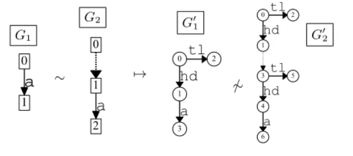
Figure 1. An Example of Unsound Encoding
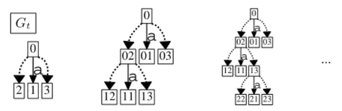
graphs: bulk semantics. With bulk semantics, a structural recursion is evaluated by first processing in parallel on all edges of the input graph and then combining the results. This bulk semantics relies on introduction ofε-edges (like ε transition in automata) to graphs, providing a smart way of treating shared nodes and cycles in graphs. In addition, UnCAL is designed carefully such that (i) every transformation is bisimulation generic in the sense that it returns bisimilar results for bisimilar inputs, and (ii) every transformation necessarily terminates and transforms finite graphs to finite graphs.
Despite its beauty in theory and usefulness in graph querying, there are two limitations in UnCAL that prevent it from being used widely. One is that UnCAL can treat only unordered graphs, being weak in other graph models, such as ordered graphs where edges from a node are ordered, which is widely used in many applica-tions: e.g., in Ecore, MOF, and KM3 [Jouault and B´ezivin 2006]. The other limitation is lack of expressive power of transformations on sibling dimension. For example, when a graph labeled with nat-ural number, we can not write in UnCAL a transformation which extracts all such edges of some node that are labeled with the aver-age number among all the siblings.
At the first sight, it seems that the first limitation could be easily solved by encoding ordered graphs by unordered ones with suitable edge labels, say usinghdandtlto represent the first branch and the rest of the branches respectively. However, there is a fatal problem with this encoding. The above encoding is unsound in the context of UnCAL whereϵ-edges must be taken into account for graph construction and structural recursion. As shown in Figure 1, the ordered graphsG1andG2, where we use dotted arrows to represent
ε-edges, are naturally bisimilar, but their corresponding encoded graphsG′
1andG′2are not at all.
... we have shown how the principles of UnQL will work on an ordered tree. However, it is not clear how they can be extended to an ordered graph model. ... we still lack a complete picture of this topic ...
In this paper, we provide a novel solution to this open problem, by defining a subtle notion of bisimilarity for ordered graph having
ε-edges so that structural recursion can be extended from that for unordered graphs to that for ordered graphs. Moreover, we propose
λT
FG, powerful higher order graph transformation languages, which
extends the lambda calculus with graph operations generalized with monads and also extended with sibling transformation.
The main technical contributions of this paper can be summa-rized as follows.
There are mainly two independent contributions; (i) one is the definition of bisimilarity for ordered graphs, which has a subtle problem of infinite width, which can not be seen in other graph models; (ii) the other one is the generalization with monadsTand extension of expressive power of graph transformations: introduc-tion of higher order funcintroduc-tion and sibling transformaintroduc-tion. Further detail of these contributions are the following:
(i). We give the first definition of the bisimilarity between ordered graphs having ε-edges, which forms the semantic foundation forλList
FG . Specifically, we identify that the branch order of even
finite graphs is not necessarily finite but countable linear order, and clarify that combination ofε-edges and cycles will induce such countable linear order on branching, which would produce new issues not occurring for the unordered case. We show that the judgment of emptiness of ordered graphs is decidable, and that it is decidable whether we can eliminate allε-edges—with keeping finite width of graph—for a finite ordered graph having
ε-edges.
(ii). UnCAL consists of the following three technical points:
• graph models and bisimilarity,
• syntactic graph representation (called graph constructors), and
• structural recursion.
We generalize all the three points with monadsT and extend further:
• We generalize the graph model in such a way that collec-tion of outgoing edges of a node has the structure of the monadT. With this, unordered graph and ordered graph correspond to finite powerset monad and list monad, respec-tively. We can see its usefulness from other examples of multiset monad and distribution monad which correspond to weighted graph and probability graph, respectively. Then we give a definition of bisimilarity for such graph models generally withT. The above (i), i.e., the definition of bisimilarity for ordered graph is independent contribution from this general definition; since for the general definition we assume existence of iteration operators, which is newly given in this paper for ordered graph, while those for other graph models are already known.
• Then according to the generalization of graph model, we also give generalized definition of graph constructors and structural recursion with monads. Specifically, we general-ize bulk semantics of the structural recursion, and show that structural recursion is bisimulation generic. The bisimula-tion genericity is a stronger result than that in [Buneman et al. 2000] even for the case of unordered graph, since here we prove bisimulation genericity of structural recursion as a higher order function, while in [Buneman et al. 2000] it
is proved as first order functions. This higher order bisimu-lation genericity enables us to introduce higher order func-tions to UnCAL and reformulation as a lambda calculus.
•We define our graph transformation languagesλT
FG as
ex-tensions of the simply typed lambda calculus, which is in sharp contrast to UnCAL (first order calculus). This refor-mulation does not only provides us higher order functions, but also a clear vision of how to extendλT
FGfurther, with
other primitive functions or other type systems such as co-product types, inductive data types, monad types, and poly-morphic types.
•We show how to overcome the second limitation of UnCAL, i.e., expressive power on sibling dimension, by introducing two sibling transformationl-sblandu-sblupon the above flexibility of extensions. For instance, whenT =List, we can manipulate branches of nodes as we transform lists: we can, for example, reverse the order of branches of a node in an ordered graph with reverse function of list.
•Summarizing the above, we formulate parametrized graph transformation languagesλT
FGwith monadsT.
(iii). Then we have the following discussion for further extension.
•We extend the structural recursion to unify the above sib-ling transformations with the extended structural recursion, so that we can transform graphs in depth-direction and in sibling-direction at the same time.
•Finally we discuss how we can systematically compose graph transformation languages to increase language power, by using monad transformer. For instance, although λList
FG
can treat ordered graphs but not unordered graphs, by this modular method, we can systematically obtainλPfin×List
FG ,
which can treat both unordered and ordered graphs.
Organization of the Paper We shall start by an overview ofλT
FG,
focusing on the case whenT = List, in Section 2. Then in Sec-tion 3, we see the first key technical contribuSec-tion of this paper, i.e., the definition of bisimilarity for ordered graphs havingε-edges. Then we give a general definition of bisimilarity for graphs inλT
FG.
In Section 4, we give interpretations of terms ofλT
FG, which
in-cludes graph constructors, structural recursion, and sibling transfor-mations; then we show their bisimulation genericity. In Section 5, we extend structural recursion with sibling transformation. In Sec-tion 6, we discuss how we can extend the languages with monad transformers. We discuss the related work in Section 7 and con-clude the paper in Section 8.
2.
Overview of
λ
TFGWe start with an overview of our general graph transformation languageλT
FG, especially whenT = List. In fact,λ
List
FG, which
treats ordered graphs, is the most important case to understand essence ofλT
FG. In the following, after giving general definition
of graphs, we will move to the case ofList, and see how ordered graphs are constructed and how structural recursion can be easily used to transform ordered graphs. In Section 4.4, we will see how to design the syntax of generalλT
FG.
2.1 Graph Model ofλT
FG
Graph inλT
FG is rooted, directed, and edge-labeled graph.
Addi-tionally, graph inλT
FG has two prominent features, ε-edges and
(a) A Simple Graph:G (b) An Equivalent
Graph:G′
1
2
d
4
d
d
3&y
b
d
(c) Result of
a2d xcon (a)
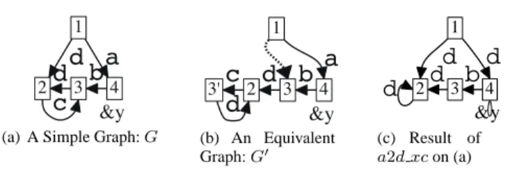
Figure 2. Examples of Graphs
We introduce the notion of graph with “T-kind of branch” for a monadT. First let us recall the notion of monad (in the Kleisli triple style):T = (T,return,lift)is a monad onSetifT:Set→Set
is a functor,
return:S→T(S)
and
lift: (S→T(S′))→(T(S)→T(S′))
are natural transformations, and they satisfy certain axioms called monad laws, see [Benton et al. 2000; Moggi 1989] for the axioms.
Example 1 (List Monad). Listis a monad defined as follows.
return(s) = [s] (s∈S)
liftf=concat◦List(f) (f:S→List(S′))
where
concat:List(List(S′))→List(S′)
is flattening a list of lists to a list.
Now we define the graph model. We useLto denote a set of
labels andLϵto denote the disjoint unionL ∪ {ε}. LetXandY
be finite sets of markers; we add the prefix&for meta-variables of markers like&x. Then aT-graph (or just graph)Gis defined as a triple(V, B, I)where
•V is a set of nodes,
•B:V →T(Lϵ×V+Y)is a branch function, where an element
xinLϵ×V+Y (called a branch) is either an edgeEdge(l, v)
or an output markerOutm(&y), and
•I:X →V is a function, which determines input nodes (roots) of the graph.
Note that in the terminology of coalgebra theory, aT-graph is a coalgebraBof the endofunctorT(Lϵ×(-)+Y)equipped with|X
|-number of initial statesI.
Example 2 (Ordered Graph). We callList-graphs ordered graphs,
where the branches are ordered. The graph in Figure 2(a) is repre-sented as(V, B, I)where
V = {1,2,3,4}
B(1) = [Edge(d,2),Edge(a,4)]
B(2) = [Edge(c,3)]
B(3) = [Edge(d,2)]
B(4) = [Edge(b,3),Outm(&y)]
I(&) = 1.
The set of graphs—withX andY as sets of input and output markers, respectively—is denoted byTDBXY, whereT may be
omitted if it is clear from context. We call aT-graph a finiteT -graph when V is a finite set, and write TDBfXY for the set of
finiteT-graphs. (“DB” is from [Buneman et al. 2000] and means “DataBase”.)
We occasionally use record notation(-).V,(-).B, and(-).Ifor components of a graph: i.e.,G= (G.V, G.B, G.I).
We allow a graph to have multiple roots: multi-rooted graph is to forest what single-rooted graph is to tree. For single-rooted graphs, we often use default marker&to indicate the root, and useDBY to
denoteDB{Y&}.
An output marker is a place holder through which the input node of another graph can be connected with anε-edge. (This is done with@,cycle(see Figure 3), andsrec(see Figure 7) to be explained later.)
Example 3 (Unordered Graph, Weighted Graph, Probability Graph). For the finite powerset monad Pfin, Pfin-graph is
un-ordered graph, which is (equivalent to) the graph model of UnCAL.
Let us consider the finite multiset monad (bag monad)Mfin:
Mfin(S)def={ϕ:S→N|ϕ−1(N−{0})is a finite set}.
Then branch ofMfin-graph has a bag semantics (rather than set
semantics ofPfin), i.e., multiplicity (called weight) of an identical
branch is not ignored.
The finite probability distribution monadDfinis defined as:
Dfin(S) def
={ϕ:S→[0,1]|ϕ−1((0,1])is a finite set,Σsϕ(s)=1}.
The monad structure is defined as below: fors∈S,return(s)is the Dirac delta function
δs:S →[0,1]
s7→1
(other thans)7→0
and forf:S→Dfin(S′),
lift(f):Dfin(S)→Dfin(S′)
(ϕ:S→[0,1])7→ (
lift(f)(ϕ):S′→[0,1]
s′7→Σs∈S(ϕ(s)·f(s)(s′))
)
Dfin-graph has probabilistic branch.
2.2 Overview ofλList
FG
From now we see an overview ofλT
FGwhenT =List.
2.2.1 Graph Equivalence
For ordered graphs, we consider bisimilarity as their graph equiva-lence, which is called value-equivalence in [Buneman et al. 2000], since we observe only “values”land&ypointed by a “pointer”v. For instance, the graphsGandG′, in Figure 2(a) and 2(b), respec-tively, are considered as being equivalent. InG′, nodes3and3′
are bisimilar because both of them only have one outgoing edge la-beleddto the node2. Also inG′, from node1to node3, there is an
ε-edge (denoted by the dotted line), which can be eliminated with keeping its bisimilarity by adding outgoing edge labeleddfrom node1to node2. Unreachable parts from roots are disregarded. The definition of bisimulation on ordered graphs withε-edges is one of the important results in this paper, and this will be addressed formally in Section 3.
A graph functionfis called bisimulation generic iff(G)and
f(G′) are bisimilar whenever G and G′ are bisimilar. λT
FG is
designed to make the interpretation of every term bisimulation generic.
2.2.2 Graph Constructors
Figure 3 summarizes the nine graph constructors used inλList
FG, and
[] 〈a : G〉
G a
G &x := G
&x
()
&x1 ... &xk
&y1 ... &yn
&x’1 ... &x’m
&y1 ... &yn
G1 G2
G1G2 G1@G2
&x1 ... &xk
&y1 ... &ym
G1
&z1 ... &zn
&y1 ... &ym
G2
ε ε
cycle (G)
&x1 ... &xm
&x1 ... &xm
ε ε
G
〈&y〉
&y G1 ++ G2
G1 G2 &x1 ... &xm
&y1 ... &yn
Figure 3. Graph Constructors
e::= x|λx.e|ee|caseeof inl(x)→eor inr(y)→e
|inle|inre|(e, e)|πle|πre {terms of lambda calculus}
|ifetheneelsee {conditional}
|a|&y|e=e {label (a∈ L), marker, and their equality}
|[]|e++e {algebraic graph constructors}
| ⟨e:e⟩ | ⟨&y⟩ |&x :=e|()|e⊕e|e@e|cycle(e)
{common graph constructors}
|isEmpty(e) { graph emptiness checking}
|srec(e)(e) {structural recursion application}
|nil|cons(e, e)|foldr(e, e, e)|... {list operators}
|l-sbl(e)(e)|u-sbl(e)(e) {sibling transformations}
Figure 4. λList
FG Language
andG1++X,YG2; however we will omit the subscriptXandY to
avoid clutter.
Let us see each constructor; also see how type discipline on in-put and outin-put markers works for each constructor. First, [] con-structs a root-only graph with the default input marker and no output markers. For two graphsG1 andG2 having identical in-put markers and outin-put markers,G1++G2adds two branchingε -edges from each new root to the corresponding old roots ofG1and
G2. Next,⟨a:G⟩extendsGwith onea-labeled edge pointing the old root from a new fresh root node; and the constructor⟨&y⟩ con-structs a graph with a single node marked with an output marker&y (in [Buneman et al. 2000],⟨a:G⟩and⟨&y⟩are denoted as{a:G} and&y, respectively). Marker renaming&x:=Gassociates an input marker&x to the root node ofG;()constructs a trivial graph that has neither a node nor an edge; andG1⊕G2constructs a disjoint union ofG1andG2, where their branching functionsB1andB2
work independently. Then,G1@G2composes two graphs sequen-tially by connecting the output nodes ofG1with the corresponding input nodes ofG2byε-edges, andcycle(G)connects the output nodes with the input nodes ofGto form cycles. It is worth noting that this set of constructors are powerful enough to describe any finite ordered graphs.
2.2.3 Syntax ofλList
FG
Our graph transformation language λList
FG (and in general λTFG)
is an extension of the simply typed lambda calculus with graph constructors and graph operations. The syntax ofλList
FG is depicted
in Figure 4, and the types and typing rules are in Figure 5. The typeDBXY is interpreted toDBfXY: the set of finite graphs,
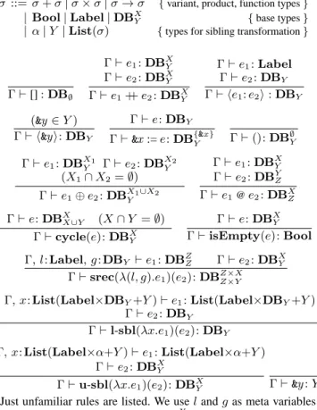
andαare type variables, which are used just foru-sbland ex-plained later. We omit the standard explanations for lambda terms, conditional, label, and equality for labels.
σ ::= σ+σ|σ×σ|σ→σ {variant, product, function types}
|Bool|Label|DBX
Y {base types}
|α|Y |List(σ) {types for sibling transformation}
Γ⊢[]:DB∅
Γ⊢e1:DBXY
Γ⊢e2:DBX
Y
Γ⊢e1++e2:DBXY
Γ⊢e1:Label
Γ⊢e2:DBY
Γ⊢ ⟨e1:e2⟩:DBY
(&y∈Y) Γ⊢ ⟨&y⟩:DBY
Γ⊢e:DBY
Γ⊢&x:=e:DBY{&x} Γ⊢():DB∅Y
Γ⊢e1:DBX1
Y Γ⊢e2:DB X2
Y
(X1∩X2=∅)
Γ⊢e1⊕e2:DBX1∪X2
Y
Γ⊢e1:DBX
Y Γ⊢e2:DBYZ
Γ⊢e1@e2:DBXZ
Γ⊢e:DBXX∪Y (X∩Y =∅)
Γ⊢cycle(e):DBXY
Γ⊢e:DBXY Γ⊢isEmpty(e):Bool
Γ, l:Label, g:DBY ⊢e1:DBZZ Γ⊢e2:DBXY
Γ⊢srec(λ(l, g).e1)(e2):DBZZ××XY
Γ, x:List(Label×DBY+Y)⊢e1:List(Label×DBY+Y)
Γ⊢e2:DBY
Γ⊢l-sbl(λx.e1)(e2):DBY
Γ, x:List(Label×α+Y)⊢e1:List(Label×α+Y)
Γ⊢e2:DBX
Y
Γ⊢u-sbl(λx.e1)(e2):DBX
Y Γ⊢&y:Y
(Just unfamiliar rules are listed. We uselandgas meta variables for variables of typesLabelandDBXY, respectively.)
Figure 5. Types and Typing Rules of UnCALList
The graph constructors here are described separately, divided into algebraic graph operators and common graph constructors. Algebraic graph operators depend onT, while the seven common graph constructors are fixed independently fromT. In fact, alge-braic graph operators further depend on signatures ofT, as seen in Section 6; but independently from choice of such signatures, their expressive power remains the same not just on closed terms but also on open terms. The boolean expressionisEmpty(e)results intruewhen the graph of the result ofehas no non-εedge in the accessible part.
Structural Recursion Now we explain structural recursion, which is a powerful mechanism borrowed from UnCAL [Bune-man et al. 2000] to describe graph transformations. The structural recursionf=srec(λ(l, g).e)is such a function thatfsatisfies the following equations, where we ignore output markers and consider the case whenXis singleton, for simplicity:
f([]) = []
f(⟨l:g⟩) = e(l, g)@f(g)
f(g1++g2) = f(g1) ++f(g2)
The above equations give a definition off as a function which inputs finite graphs and outputs infinite graphs, in recursive way. However the outputs offare in fact (bisimilar to) finite graphs, and it is made clear by the bulk semantics off, which will be given in Section 4.2. Intuitively, in the bulk semantics, structural recursion
Example 4. The following structural recursiona2d xcreplaces all labelsawithdand contracts edges labeledc.
a2d xc=srec(rc) where
rc=λ(l, g).if l=athen⟨d:⟨&⟩⟩
else if l=cthen⟨&⟩
else⟨l:⟨&⟩⟩
Applying the functiona2d xcto the graph in Fig. 2(a) yields the graph in Fig. 2(c).
Example 5. Consider an ordered graph representation of books. Since “sections” are ordered and there are some reference links in books, we can see books as ordered graphs. The following struc-tural recursiontoc, which is adapted from [Robertson et al. 2009], computes the table of contents of books in which sections can be arbitrarily nested:
toc(db) =srec(λ(l, g).ifl=section
then⟨section: (get title(g) ++⟨&⟩)⟩
else⟨&⟩) (db)
where the functionget titleresults in the title of the section.
get title(g) =srec(λ(l1, g1).if l1=title
then⟨title:srec( λ(l2, g2).⟨l2:[]⟩ ) (g1)⟩
else[]) (g)
Sibling Transformation Structural recursion functions are pow-erful transformations which terminate at evaluation and preserve finiteness of graphs, but we need more expressive power: transfor-mations on sibling dimension.
Let us consider an ordered graph and its unfolded (maybe infi-nite) tree. The branches under the root are then a list of the subtrees. Then if one wants to, e.g., reverse the order of the branches under the root, we can not do so with the structural recursion.
To resolve this problem, we introduce local sibling
transforma-tionsl-sbland uniform sibling transformationsu-sbl, which en-able such transformations. The formerl-sbltransforms branches only of the root node of a single-rooted graph; and by combination with the structural recursion,l-sblcan transform branches of any one node which the structural recursion function can reach. The latteru-sbltransforms branches uniformly of all nodes in a graph. Let us return to the Figure 4. List operators in the syntax are usual ones; we can add anything that is convenient such ascar,
cdr, filter, and reverseetc. These list operators are used for the two sibling transformations; l-sbl(λx.e) and u-sbl(λx.e)
transform sibling asλx.e transforms lists. In the typing rule for
u-sbl, we use type variables α to prepare a parametric poly-morphic functionλx.eonList(Label×α+Y)so thatλx.eand hence u-sbl(λx.e) become “uniform” on α. The parametricity guarantees bisimulation genericity of u-sbl. For the detail see Section 4.3.
3.
Bisimilarity for
ε
-edge and Ordered Graph
Section 2.1 gives a general definition ofT-graph, for a monadT. To this end, we shall give the semantic equivalence for the graph model ofλTFG: bisimilarity betweenT-graphs.
The main point is a treatment ofε-edge. The case of ordered graph (List-graph) involves a big problem which does not occur for unordered graph (Pfin-graph): i.e.,ε-elimination might induce
infinite width. In the following, we shall see the problem and
how to define bisimilarity between ordered graphs. Also we give some effective procedure to avoid such infinite width. Then we
Gs
0
1
a
∼00
10 01
a
... 11
a
∼...
00
01
a
11
a
Gb
0
1
a
∼00
10 01
a
20
...11
a
... ...21
a
... ∼
00
... 11
a
... 01
a
... 21
a
...
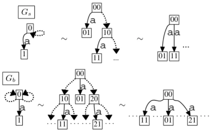
Figure 6. Graphs with Stream Branching and with Dense Branch-ing
give a general definition of bisimilarity forT-graphs. Finally, we extend the bisimilarity equivalence from graph types to higher order function types.
We here remark that our bisimilarity for the invisible label ε
is different from weak bisimilarity for the invisible labelτ in the context of process algebra [Milner 1999]. Our bisimilarity is char-acterized by theε-elimination (Proposition 8.2) which is familiar in automata theory. One purpose of our use ofε-edge is to post-pone calculation of graph constructors, structural recursion and so on, but weak bisimilarity is unsuitable with respect to properties of such graph transformations: e.g. associativity of++fails with weak bisimilarity.
3.1 Bisimilarity for Ordered Graph
Now we see the bisimilarity between ordered graphs: its intuition and formal definition.
Intuition of the Bisimilarity
First let us see some examples of ordered graphs in order to have some feeling of the bisimilarity to be defined. Consider the graphs in Figure 6. For the graphGs, first, in order to make our problem
easily understandable, let us unfold the graph to an infinite tree, i.e., the graph in the middle. Then intuitive “ε-elimination” of the tree is the graph on the right, where the branching is as a stream. Note that for ordered graph there is no idempotency which unordered graph has. The way of branching of graphs having ε-edges are thus possibly infinite essentially. However, it is not necessarily just a stream type, as in the next example Gb. Unfolding of graph
Gb yields the tree in the middle, and then its “ε-elimination” is
the graph on the right. This graph has a branch like the ordered set{n/2m
∈Q|n, m∈N,0<n<2m
}, which is a dense countable linear ordered set. (In this paper, the term countable includes the case of finite.)
In fact, for any countable linear ordered set, there is some ordered graph havingε-edges such that the branches of the root after eliminatingε-edges are exactly as the given ordered set. (For the detail, see Appendix A.)
Formal Definition of the Bisimilarity
Now let us define bisimilarity between ordered graphs. As seen above, theε-elimination of an ordered graph might induce count-able width. So we shall first define a generalized notion of “ordered graph with countable width”, and define bisimilarity for such gen-eralized graphs. This asks us to extend the list monad
List(S)def= Σn∈NS
to the countable list monad CList which can be defined as the following:
CList(S)def= ΣL∈LS
L
whereNis generalized toL, the set of countable linear ordered sets up to order isomorphism (with chosen representativesL). (See Appendix B for the precise definition ofCList.) Thus we extend ordered graphs toCList-graphs.
ForB(v) ∈ΣL∈L(Lϵ×V+Y)L, let|B(v)|denote the
count-able linear ordered setL ofB(v). Then, we call i ∈ |B(v)|a branch index of a nodev, and writeB(v).i∈ Lϵ×V+Y for the
i-th branch.
Next we prepare the notion of “transitive closure” ofε-edges. LetG= (V, B, I)∈ CList DBXY andv ∈V. Let us consider a
pair of anε-path fromvand a branch indexinof the last node in
theε-path:
v(=v0)→εi0 v1...
ε
→in−1vn→in(n∈N)
wherevn→inmeans just thatin ∈ |B(vn)|. We call this proper
branch ofvif thein-th branchB(vn).inis not anε-edge, i.e., it
is either a non-εedge or an output marker. The set of all proper branches ofvinGis denoted byPb(G, v). It is easily shown that
Pb(G, v)is a countable set.
Then there is a natural linear order≤PbonPb(G, v): for two
different proper branches
p= (v→εi0v1...
ε
→in−1vn→in),
p′= (v→εi′
0v
′
1...
ε
→i′
n′ −1v
′
n′→i′
n′),
we obtain their branch indices sequences:p˜ def= (i0, ..., in−1, in)
and p˜′ def= (i′0, ..., i′
n′−1, i′n′). With the starting node v, we can
recoverpandp′ from these indices sequences. Then, betweenp˜
andp˜′, we can consider lexicographical order≤l, then we define
p≤Pbp′⇐⇒def p˜≤lp˜′.
Now we define the bisimilarity.
Definition 6 (Bisimilarity). ForCList-graphsG= (V, B, I), G′=
(V′, B′, I′) ∈ CList DBX
Y, a relationR betweenV andV′ is
called a bisimulation relation if for anyvRv′, there is an order iso-morphismf: (Pb(G, v),≤Pb) → (Pb(G′, v′),≤Pb)satisfying
the following property. For any proper branch
p= (v→εi0 ... vn→in)∈Pb(G, v)
with
f(p) = (v′→εi′
0... v
′
n′→i′
n′)∈Pb(G
′, v′),
•ifB(vn).in =Edge(l, u)for somel ∈ L, u∈V, then there
existsu′∈V′such thatB′(v′
n′).i′n′=Edge(l, u′)anduRu′,
•ifB(vn).in=Outm(&y)for some&y∈Y, thenB′(vn′′).i′n′=
Outm(&y).
Two graphsGandG′are bisimilar (denoted byG∼G′) if there is a bisimulation relationRsuch that for every input marker&x ∈X,
I(&x)R I′(&x).
Note that the bisimulation relation is an equivalence relation on CList DBX
Y. Next, let us defineε-elimination.
Definition 7 (ε-elimination). For aCList-graphsG= (V, B, I)∈
CList DBXY, ε-elimination ε-elim(G) of G is a CList-graph (V, B′, I) ∈ CList DBX
Y where |B′(v)|
def
= Pb(G, v) and for
p= (v→εi0... vn→in)in|B ′(v)
|,B′(v).p=defB(vn).in.
Note that theε-elimination does not change sets of nodes.
Proposition 8. 1. For all CList-graphs G ∈ CList DBX
Y,
ε-elim(G) has no ε-edge, andG andε-elim(G) are
bisim-ilar.
2. ForCList-graphsG, G′∈CList DBX
Y,GandG′are bisimi-lar if and only ifε-elim(G)andε-elim(G′)are bisimilar. Here we first gave the definition of bisimilarity for graphs hav-ing ε-edges and then gave that of ε-elimination and the above proposition. However, we can define the bisimilarity for graphs havingε-edges by the equivalence stated in Proposition 8.2 with the
ε-elimination and with the bisimilarity for graphs having noε-edge; the latter can be easily derived from general coalgebraic definition of bisimilarity [Rutten 2000]. Then we see that such definition is not just equivalent to but almost the same as that in Definition 6. Thus we find that the key here is the definition ofε-elimination. In the following we give a general definition of bisimilarity forT -graphs byε-elimination.
3.2 Decidability for Finite Width Graphs
Before going to the general setting with monadsT, we give one important decidability result forCList-graphs.
Let FG/εbe the set of finiteList-graphs which are bisimilar to some finiteList-graphs having noε-edge. There is a procedure which answers, for a finiteList-graphG, ifGis in FG/εor not. IfGis in FG/ε, we can effectively eliminateε-edges; otherwise, it is impossible to eliminateε-edges, keeping finite width. This pro-cedure is as the following. First note that for each node accessible from a root, we can check if there is anε-cycle—a cyclic path con-sisting only ofε-edges—on the node. Then if, for every accessible node withε-cycle, there is no proper branch, then the input graph is in FG/ε; otherwise, not in FG/ε.
This is enough for run-time use of the query languageλList
FG,
because, though we needε-edge for implementation—for structural recursion and for efficiency of graph calculation—practical graphs in the real world has noε-edge. If a user of the language writes such a practical query, then the result should return a graph in FG/ε; if it is an incorrect query not intended by the user, and then if the result has inevitableε-edges, the procedure above can check it and can warn the user.
Note that, in the class FG/ε, since we can eliminateε-edges, we can obtain familiar effective procedures for bisimilarity-checking and for obtaining the minimum graphs in a similar way to un-ordered graph. Also note that ifGis not in FG/ε, thenGis not empty, henceisEmptyis decidable.
3.3 Generic Definition of Bisimilarity
Now we define the notion of bisimilarity in general forT-graphs. We define this bisimilarity for any monadTwhose Kleisli category
SetThas a uniform iteration operator.
For a monad T on Set, the Kleisli category SetT of T is
defined as below: objects inSetTare sets, and morphismsS→S′
are functionsS→T(S′). The identity morphismidonSis id def=return:S→T(S),
and the compositiong◦foff:S→T(S′)andg:S′→T(S′′) is defined as
g◦fdef=lift(g)◦f:S→T(S′′).
A Kleisli category has coproducts: the coproduct ofS1 andS2is justS1+S2, and the injections are
inl
def
=return◦inl:S1→T(S1+S2)
inr
def
Copairing of a pair of functionsf1:S1 → T(S′)andf2:S2 →
T(S′)is the same as the copairing inSet, i.e.,
[f1, f2]:S1+S2→T(S′).
We write∇:S+S → T(S)and +for the codiagonal and the coproduct on morphisms inSetT, respectively.
Next we recall the notion of iteration operator [Haghverdi 2000; Kakutani 2002], which is the dual notion of fixed point opera-tor [Simpson and Plotkin 2000]; also, iteration operaopera-tor is to while operator as coproduct type is to the boolean type. Though iteration operator can be defined for any category with finite coproducts, we here define directly on the Kleisli categorySetT of a monadTon Set. An iteration operatoriteronSetTis a function which maps
a function
f:S→T(S+A)
to
iter(f):S→T(A)
such that the mapping satisfies the following axioms:
•(naturality:) forf:S→T(S+A)andg:A→T(A′),
g◦iter(f) =iter((idS+g)◦f):S→T(A′), •(dinaturality:) forf:S→T(S′+A)andg:S′→T(S+A),
[iter([f,inr]◦g),idA]◦f=iter([g,inr]◦f):S→T(A)
•(unfolding:) forf:S→T(S+A),
iterf= [iterf,idA]◦f:S→T(A),
•(codiagonal:) forf:S→T(S+S+A),
iter(iterf) =iter((∇+idA)◦f):S→T(A).
Further, iter is called uniform if for functionsf:S → T(S′),
g:S′→T(S′+A)andh:S→T(S+A), iter(g)◦f=iter(h):S→T(A)
whenever
g◦f= (f+idA)◦h:S→T(S
′+A).
The axiom of uniformity is used for logical relation for iteration operator [Hasegawa 2002]. We use uniformity to show that strong bisimilarity implies bisimilarity.
The following characterization ofε-elimination as iteration op-erator is due to [Hasuo 2011; Jacobs 2010a].
Definition 9 (ε-elimination). LetTbe a monad anditerbe an
iter-ation operator inSetT. For anT-graphG= (V, B, I)∈TDBXY,
its ε-elimination ε-elim(G) ∈ TDBXY is (V, B′, I) where
B′ def
= embed ◦iter(iso ◦B); here embed is the embedding
T(L×V+Y)→T(Lϵ×V+Y), andisois the composition of
T(Lϵ×V+Y)∼=T((L+1)×V+Y)∼=T(V+(L×V+Y)).
Conversely, ε-elimination induces an iteration operator; let us consider a T-graph (V, B, I) in the case whenL= 0. Then
B:V → T({ε}×V+Y), and if we applyε-elimination, the re-sulting branch function isB′:V →T(0×V+Y). That is, we get an operator which maps a functionV →T(V+Y)to a function
V →T(Y). This is just the same as the structure of an iteration operator in the Kleisli category (if we allow Y to be arbitrary sets); and we find that it is natural to adopt the axioms of iteration operator also as axioms ofε-elimination.
Now we give a general definition of bisimilarity forT-graphs, using the aboveε-elimination.
Before that, let us recall the notion of bisimulation relation for general endofunctorF onSet. First we recallF-lift of relations:
for (the inclusion function of) a relation r:R ֒→ V×V′, let
r1def=prl◦R:R→V andr2
def
=prr◦R:R→V′; so
⟨F(r1), F(r2)⟩:F(R)→F(V)×F(V′).
ThenF˜(R)is defined as the image
⟨F(r1), F(r2)⟩(F(R))⊆F(V)×F(V′).
For a functorF onSet, and two coalgebras ofF, i.e., two func-tionsB:V → F(V)and B′:V′ → F(V′), a bisimulation
re-lationRbetweenB andB′ is a relationR ⊆ V×V′such that
(B×B′)(R)⊆F˜(R).
Definition 10 (Strong Bisimilarity and Bisimilarity). LetT be
a monad, and G = (V, B, I) and G′ = (V′, B′, I′) be T -graphs inTDBXY. Then Gand G′ are strong bisimilar if there
is a bisimulation relationRw.r.t. the endofunctorT(Lϵ×(-)+Y)
betweenBandB′such that for any&x ∈X,I(&x)R I′(&x). Now let iter be a uniform iteration operator in SetT. Then
GandG′ are bisimilar (written asG ∼ G′) if ε-elim(G) and
ε-elim(G′)are strong bisimilar.
Note that the notions ofε-elimination and bisimilarity depend on a given iteration operator, but in this paper we do not refer the dependency in the terminology.
We assume that all monads T in the paper preserve weak-pullbacks, which is just a mild assumption often used in coalgebra theory [Rutten 2000; Sokolova 2005]. Especially, thenT preserves injections and finite intersections. Using this assumption, it is eas-ily checked that the strong bisimilarity relation is an equivalence relation onTDBX
Y.
It is immediately shown that strong bisimilarity implies bisim-ilarity from the uniformity of an iteration operator. We use this property in some proofs in the papers. (In fact we can weaken the assumption of uniformity to that of uniformity with respect to
mor-phisms inSet[Simpson and Plotkin 2000, Definition 2.7].) Thus we gave the definition of bisimilarity, but it is not neces-sary that every monad has an iteration operator in the Kleisli cat-egory. However, as the case ofList withCList, there is the case that a monadTis presentable in programming languages, does not have iteration operator, and has an extensionT′which might not be presentable in languages but has a uniform iteration operator. We say thatThas an extensionT′forε-elimination if there is a monad
T′, an injective monad morphismι:T ֒→T′, and a uniform iter-ation operator in the Kleisli category ofT′. Here monad morphism is a natural transformation which is compatible withreturn’s, and withlift’s (see [Benton et al. 2000], for the detail).
By this, we generalize the definition of bisimilarity:
Definition 11 (Bisimilarity Generalized on Size). Let T be a
monad which has an extensionT′ forε-elimination. Then there is the embedding ι-DBXY:TDB
X
Y ֒→ T′DB X
Y which maps (V, B, I) to(V, ι(Lϵ×V+Y)◦B, I). ForGand G′ in TDBXY,G andG′are bisimilar ifι-DBX
Y(G)andι-DBXY(G′)are bisimilar
in the sense of Definition 10.
By the assumption that ι has injective components and
T preserves weak pullback, ι-DBX
Y reflects strong
bisimilar-ity [Sokolova 2005, Theorem 4.3.6], and hence forT-graphs hav-ing noε-edges, strong bisimilarity and the above bisimilarity are equivalent.
f:S→Pcnt(S+S′),
iter(f)(s)def= ∪ n∈N
(f2◦(f1)n)(s)),
where
f1def= [idS,const{}]◦f:S→Pcnt(S) f2def= [const{},idS′]◦f:S→Pcnt(S
′
)
and then-times composition(f1)n
is that inSetPcnt.
Similarly, finite multiset monadMfin has an extension for ε
-elimination, i.e., countable multiset monadMcnt:
Mcnt(S) def
={ϕ:S→N∪{∞} |ϕ−1(N−{0})is countable}.
The iteration operator forMcntis given with the same formula as
that forPcnt.
Also finite probability distribution monadDfinhas an extension
forε-elimination, i.e., countable subprobability distribution monad SubDcnt:SubDcnt(S)
def
=
{ϕ:S→[0,1]|ϕ−1((0,1])is countable,Σxϕ(x)≤1}.
Note that here the summation of probabilitiesΣxϕ(x)is not
neces-sarily 1; this is because the probability1−Σxϕ(x)is reserved for
that of the abort of the iteration operator. The definition of the it-eration operator forSubDcntis also similar to those forPcntand
Mcnt, see [Jacobs 2010b] for the detail.
ForListwithCList, conversely rather we can give the iteration operator inSetCList with theε-elimination in Definition 7 in the
way described after Definition 9.
3.4 Bisimilarity for Higher Order Functions
So far we have given the semantics for base types, i.e., bisimilarity for graph typesDBX
Y, and give just equality relations for the other
base types. Here we extend such equivalence relations for base types to higher order function types.
It is well known that if we want to lift equivalence relation to function types then we need to switch from the notion of equiva-lence relation to that of partial equivaequiva-lence relation, i.e., an equiv-alence relation on some subset of an original set. This is because, now not all functions onDBfXY are bisimulation generic, so we
have to cut out the subset consisting of bisimulation generic func-tions.
Now let us see the formal definition. Letσbe a type ofλT
FG.
We define binary logical relation∼σfrom the above equivalence
relations on the base types. Let us recall the logical relation∼σ
only on the essential case, i.e., function type:σ =σ1 →σ2. By induction hypothesis, we already defined a binary relation∼σion
[[σi]]. Then we define a binary relation∼σon[[σ]]
def
= [[σ1]]→[[σ2]]
as
f∼σf′⇐⇒ ∀def x, x′∈[[σ1]].(x∼σ1 x
′
⇒f(x)∼σ2f
′(x′))
⇐⇒ ∀x∈ |∼σ1|. f(x)∼σ2f
′(x).
Then for any typeσ,∼σbecomes a partial equivalence relation
on[[σ]], i.e., an equivalence relation on the subset
|∼σ|
def
={x∈[[σ]]|x∼σx}.
We call a functionf: [[σ1]] → [[σ2]] (higher order) bisimulation generic iffis in|∼σ1→σ2|, i.e.,
∀x, x′∈[[σ1]].(x∼σ1x
′
⇒f(x)∼σ2 f(x
′)). Then by the Basic Lemma of logical relation, interpretations of all the terms are bisimulation generic if interpretations of all the constants are bisimulation generic; and then we obtain a
model ofλT
FGin the cartesian closed categorySet, see the
text-book [Mitchell 1996] for the detail. Note that the above lifting to function types is possible for any equivalence relations such as strong bisimilarity.
In the next section we show the bisimulation genericity for all constants.
4.
UnCAL Generalized with Monad
In this section we give interpretations of terms ofλT
FGand show
their bisimulation genericity. As explained in the last of the previ-ous section, it is enough to consider only constants; we will see graph constructors, structural recursion, and sibling transforma-tions. In the last place, we see how to define syntax ofλT
FG.
4.1 Graph Constructors
UnCAL andλList
FG respectively have nine graph constructors, as in
Section 2.2.2, by which we can represent all finite graphs. Here we define such graph constructors forT-graphs by which we can represent all finiteT-graphs.
Among the nine graph constructors ofλList
FG, [] and++are
in-herent in the list monadList, and the other seven constructors are common for all monads.List(S)is free monoid (generated by a set
S), which has nullary and binary operations: unit and multiplica-tion. The nullary graph constructor [] and binary graph constructor
++correspond to the unit and the multiplication, respectively. First we define the seven common graph constructors for T -graphs.
Definition 13 (Common Graph Constructors).
• ForG= (V, B, I)∈DBY,
⟨l:G⟩def= (V ∪ {v0:fresh}, B′,{&7→v0})∈DBY
B′def=B∪ {v07→return(Edge(l, I(&)))}. • ForG= (V, B, I)∈DBY,
(&x:= G)def= (V, B,{&x7→I(&)})∈DB{Y&x}.
• For&y∈Y,
⟨&y⟩def= ({&}, {&7→return(Outm(&y))},id{&})∈DBY.
• ()def= (∅, ∅,id∅)∈DB∅Y.
• ForG= (V, B, I)∈ DBX
Y andG′ = (V′, B′, I′) ∈DBX
′
Y
such thatX∩X′=∅,
G⊕G′def= (V+V′, B′′, I+I′)∈DBXY∪X′
B′′def= [T(Lϵ×(inl)+Y)◦B, T(Lϵ×(inr)+Y)◦B′]
:V+V′→T(Lϵ×(V+V′)+Y).
• ForG= (V, B, I) ∈ DBX
Y andG′ = (V′, B′, I′) ∈ DBYZ,
G@G′def
= (V+V′, B′′, in
l◦I)∈DBXZ where
B′′(inl(v))
def
=lift(f)(B(v))
f:Lϵ×V+Y →T(Lϵ×(V+V′)+Z) Edge(l, v)7→return(Edge(l,inl(v)))
Outm(&y)7→(T(Lϵ×(inr)+Z))(B′(I′(&y)))
B′′(in
r(v′))
def
= (T(Lϵ×(inr)+Z))(B′(v′)).
• For a graphG = (V, B, I) ∈ DBX
X∪Y whereX∩Y = ∅, cycle(G)def= (V, B′, I)∈DBX
B′(v)def
=T(f)(B(v)).
f:Lϵ×V+(X∪Y)→ Lϵ×V+Y Edge(l, v)7→Edge(l, v) Outm(&x)7→Edge(ε, I(&x)) Outm(&y)7→Outm(&y)
In the definition ofB′′(inl(v))in the definition of@, by
replac-inglift(f)(B(v))withT(f′)(B(v))where
f′:Lϵ×V+Y → Lϵ×(V+V′)+Z Edge(l, v)7→Edge(l,inl(v))
Outm(&y)7→Edge(ε, I′(&y))
we obtain@′operator, which is bisimilar to@operator. With@
operator, we find that we do not needε-edge for graph constructors except forcycle, but@′is useful to postpone extra calculation of
@, which is in effect equivalent to one step ofε-elimination. We note that the multi-rootedness is semantically the same as power of sets of graphs (or tuple of graphs):DBfXY ∼= (DBfY)
X
. The functionDBfXY →(X →DBfY)isG7→(&x7→ ⟨&x⟩@G),
and the inverse is
f7→(&x1:=f(&x1))⊕...⊕(&xn:=f(&xn))
when X = {&x1, ...,&xn}. Still multi-rootedness is useful for
efficient implementation, i.e., to share bisimilar nodes and to save the size of graphs as small as possible.
Now we define the other graph constructors which depend on each monadT. For Proposition 19 and so on, we finally assume that a monadT is finitary; though we can postpone the definition of finitary monad till Proposition 19, we first explain finitary monad so that the reader has more concrete intuition in the following definitions and propositions.
A finitary monad on Set is a monad T on Set such that the functorT preserves all directed colimits inSet. We use this property only in the following form (and an equivalent condition explained soon): for any set S, and any x ∈ T(S), there is a finite subsetS′ ⊆ S such that x ∈ T(S′). The monads P
fin,
List, Mfin, and Dfin are all finitary monads; for example, for
[4,1,6,4,6,4]∈ List(N), we have a finite subset{4,1,6} ⊆N
and [4,1,6,4,6,4]∈List({4,1,6}).
Next we recall one equivalent condition of finitary monadT: shortly speaking,Tis generated by finite arity algebraic operations. For a monad T onSet, an elementf ∈ T(A) can be seen as an|A|-ary algebraic operation onT(S)for anyS ∈ Set: for
g∈T(S)A
, b
f(g)def=lift(g)(f)∈T(S).
For example, whenT =Pfin, forf ={0,1} ∈Pfin({0,1})and g0, g1∈Pfin(S),
b
f(g0, g1) =lift(07→g0,17→g1)({0,1}) =g0∪g1,
i.e.,{\0,1}=∪.
For a monad T, let us take a family of sets Σ(n) ⊆ T(n)
(n∈N), where we regardnas the set{0, ..., n−1}. Let us define
TΣ(i)(S)⊆T(S)(S∈Set) by induction oni∈Nas below:
TΣ(0)(S)def=return(S)⊆T(S)
TΣ(i+1)(S)=def{fb(g)∈T(S)|m∈N, g∈(TΣ(i)(S))mf
∈Σ(m)}.
Then a monadT is finitary if and only if there is aΣsuch that
T(S) =∪ i∈N
TΣ(i)(S),
and in this case, we call suchΣa family of signature sets ofT and we call elements inΣ(n)signatures.
Example 14. The three monadsPfin,Mfin, andListcorrespond
to (upper) semilattice, commutative monoid, and monoid, respec-tively; then their zero ary operations and binary operations corre-spond to signatures as below.
ForPfin,
Σ(0)def={{}} ⊆Pfin(0)
Σ(2)def={{0,1}} ⊆Pfin(2)
Σ(n)def=∅ (for othern).
For{} ∈Σ(0),c{}={} ∈Pfin(S), and as seen above,
\
{0,1}=∪:Pfin(S)2→Pfin(S).
Then any element inPfin(S)can be represented as a composition
of these operators and singletons, i.e., elements inreturn(S): e.g. {a, b, c}= ({a} ∪ {b})∪ {c}.
ForMfin, similarly,
Σ(0)def={{}} ⊆Mfin(0)
Σ(2)def={{0,1}} ⊆Mfin(2)
Σ(n)def=∅ (for othern).
Here{}and{0,1}are regarded as multisets. ForList, similarly again,
Σ(0)def={[]} ⊆List(0)
Σ(2)def={[0,1]} ⊆List(2)
Σ(n)def=∅ (for othern).
ForDfin,
Σ(2)def={sigr: 2→[0,1]|r∈[0,1]} ⊆Dfin(2)
Σ(n)def=∅ (for othern)
wheresigris defined assigr(0)def= randsigr(1)def= 1−r. Then forϕ1, ϕ2:S → [0,1] in Dfin(S), sigdr(ϕ0, ϕ1) ∈ Dfin(S) is
d
sigr(ϕ0, ϕ1):S→[0,1]such that
d
sigr(ϕ0, ϕ1)(s) =r·ϕ0(s) + (1−r)·ϕ1(s).
Now recall that “singletons” inDfin(S), i.e., elements inreturn(S)
are given as the Dirac delta functionsδsas in Example 3. Then it
is easy to see that the above family becomes a family of signature sets; for example,ϕ:N→[0,1]inDfin(N)such that
ϕ(0) = 1
2, ϕ(1) =
1
6, ϕ(2) =
1 3,
ϕ(n) = 0 (for othern),
can be represented by signatures and “singletons” as
ϕ=1
2δ0+
1
6δ1+
1 3δ2
=1
2δ0+
1 2(
1
3δ1+
2 3δ2) =sigd1
2(δ0,sigd13(δ1, δ2)).
The above family of signature sets ofDfin has infinitely many
signatures. Still, when implementingλT
FG in a programming
lan-guage, one can represent it as the image of a function. For exam-ple, first let us interpretDfin(S)asFinSet(S×Float)(or with
is regarded as a relation rather than a function, then a probability
f(s) ∈ [0,1]can be regarded as the sum of the multi values of
f(s). Then the family of signature setsΣforDfinis presented as sig:Float→Dfin(Nat)defined as below:
let sig r = {(0,r), (1,1-r)}
Now we define a graph constructor forT-graphs for each alge-braic operator ofT, i.e., for each element inT(A). Before this, note that in the definitions of graph and common graph constructors, we can easily extend set of marker from finite to arbitrary setA, and⊕ from binary operator toA-ary operator:⊕: (DBX
Y)A
∼=
→DBA×X
Y .
These are used in the following definition, but the reader who is interested only in finiteA’s—which are enough for implementable language—may apply the following simply to the caseA=n =
{0, ..., n−1}.
Definition 15 (T-Algebraic Graph Constructors). Let T be a
monad onSet. Forf ∈T(A) (A ∈Set), and a finite setX, let
GX f
def
= (X, B,id)∈DBX
A×Xwhere
B(&x)def=T(g)(f)∈T(Lϵ×X+A×X),
g:A→ Lϵ×X+(A×X)
&a7→Outm((&a,&x)).
Then we define aT-algebraic graph constructorf: (DBXY)A→
DBXY. For(Gi)i∈A∈(DBXY) A
,f((Gi)i)
def
=GX
f @(⊕((Gi)i)).
We callT-algebraic graph constructors and the common graph constructors graph constructors.
Example 16. WhenT =List, let us considerf= [0,1]∈Σ(2)
in Example 14. Let us see the picture ofG1++G2in Figure 3. This is the@′version of[0,1](G1, G2). The topm-roots areG[0,1]and
theε-edges are those by@′; and one can find that the juxtaposition of two graphs G1 andG2 inG1 ++G2 are the same as that in
G1⊕G2in the same figure.
Proposition 17. LetT be a monad onSetwith an extension for
ε-elimination. Forf ∈ T(A) (A ∈Set), andfi ∈ T(Ai) (i∈
A, Ai∈Set), let
⨿
i∈Afi:A(
∼
=⨿i∈A1)→T(
⨿
i∈AAi)
be the coproduct of the morphismsfi: 1→ T(Ai)in the Kleisli categorySetT. Then
f((fi(-))i∈A): ∏i∈A(DB X Y)
Ai→DBX
Y
is bisimilar to
lift(⨿
i∈Afi)(f): (DB X Y)
⨿
i∈AAi →DBX
Y, via the isomorphism
∏
i∈A(DB X
Y)Ai∼= (DBXY)
⨿
i∈AAi.
Hence, ifTis further a finitary monad with a family of signature setsΣ, the graph constructorfof anyf∈T(A)is a composition of the graph constructors of a finite number of some signatures in Σ.
At the same time, when we add graph constructors of all the sig-natures in one family of signature sets to a calculus, then expressive power on graph constructors are the same independently from the choice of families of signature sets.
Proof. ForGi
i′= (Vii′, Bii′, Iii′) (i∈A, i′∈Ai),
f((fi((Gii′)i′))i).V =X+Σi∈A(X+Σi′∈A
iV
i i′)
and
lift(⨿
i∈Afi)(f)((G i
i′)(i,i′)).V =X+Σ(i,i′)∈⨿
i∈AAiV
i i′.
In the former there are extraA-copy ofX, i.e.,Σi∈A(X)than the
latter; but with@(rather than@′) in Definition 15, the nodes in
Σi∈A(X) in the former are not reachable from the roots in the
former graph, so can be ignored.
The second and third points are immediate from the first point by the definition of a family of signature sets of a finitary monad.
This proposition also implies thatT-algebraic graph construc-tors obey the same axioms as those of algebra ofT. For exam-ple, finite powersets are free algebras of upper semilattice, hence the graph constructors{}and(-)∪(-)satisfy all axioms of upper semilattice: i.e., associativity, unitality, commutativity, and idem-potency.
Proposition 18 (Bisimulation Genericity of Graph Constructors).
All the graph constructors (including@′) are strong-bisimulation generic and also are bisimulation generic.
Proof. It is obvious that they are strong-bisimulation generic. Then,
for a graph constructor f, prove that ε-elim(f(G1, ..., Gn)) is
bisimilar toε-elim(f(ε-elim(G1), ..., ε-elim(Gn))). (For the case
ofcycle, use unfolding axiom of iteration operator.) This implies that strong-bisimulation genericity implies bisimulation genericity.
The next proposition is the most important property of the graph constructors, for which we requireTto be finitary.
Proposition 19 (Full-Representability). LetTbe a finitary monad
onSet which has an extension for ε-elimination. Any finite T -graphs can be constructed by the graph constructors.
Proof. The proof is basically the same as that for UnCAL
[Bune-man et al. 2000]. See Appendix D for the detail.
4.1.1 Remark on Representability of Monads
We give an important remark on “representability” of monads in languages, which explains why we need care to infinite width for List-graphs, and why we do not need such special care forPfin
-graph.
For T with an extension for ε-eliminationT′, we definedε -elimination for any T-graphs, but in fact it is enough to define
ε-elimination for finiteT-graphs, since our languages target only finite graphs. IfT is finitary, in order to defineε-elimination only for finiteT-graphs, without loss of generality we can replace the extensionT′with its finitary partT′|fin:
T′|fin(S)def=∪S′∈Pfin(S)T
′(S′). (See Appendix C for the detail why generality is not lost.)
Then,(Pcnt)|fin is equal to Pfin, hence we do not needPcnt
forλPfin
FG anymore. On the other hand,CList|fin(S) consists of
countable listslsuch that the number of elements inSwhich occur in onel are finite. For example, [0,1,0,1, ...] ∈ CList|fin(N),
but[0,1,2,3, ...] ∈/ CList|fin(N), ThusCList|fin is far different
fromList; we can not avoid the use of the notion of countable linear ordered set. (However the authors do not know if for arbitrary countable linear ordered setLthere is an finiteList-graphGwhose
ε-elimination involvesL; though we found suchGas infiniteList -graphs as in Appendix A. As in Figure 6, it is certain that a dense countable linear ordered set (and more countable linear ordered sets concatenated further) occur.)
For the other two examples,
and(SubDcnt)|fin is the finite subprobability distribution monad
SubDfin:
SubDfin(S) def
={ϕ:S→[0,1]|ϕ−1((0,1])is finite,Σxϕ(x)≤1}.
Here(Mcnt)|finand(SubDcnt)|finare representable in a language
for implementingλT
FG in a similar way to that after Example 14,
while it seems difficult to represent whole ofCList|fin, because of
the notion of countable linear ordered set.
Note the difference between being finitary and being “rep-resentable”, and also note the difference between being “repre-sentable” ofT and that ofT′. (On the other hand, recall that as above ifT is finitary thenT′can be finitary.) As above, it is not clear that being finitary of a monad implies that the monad is “representable” in a language; and being finitary ofT is used to prove the property that every term inλT
FGpreserves finiteness (of
nodes) of graphs, while “representability” ofT is needed for syn-tax of graph constructors and implementation of the graph model
B:V →T(Lϵ×V+Y). On the other hand, “representability” of
T′is needed for representation of graphs withoutε-edges, which is important if, in an application, graphs observable from users of
λT
FG should beε-edge free; in order to resolve this problem, we
gave the effective procedure in Section 3.2 for the case ofListwith CList.
4.2 Structural Recursion
Now we give a general definition of the structural recursion, which is the most important transformation method ofλT
FG. In [Buneman
et al. 2000], there are two semantics for the structural recursion: bulk semantics and memoized recursive semantics. Here we gener-alize the bulk semantics.
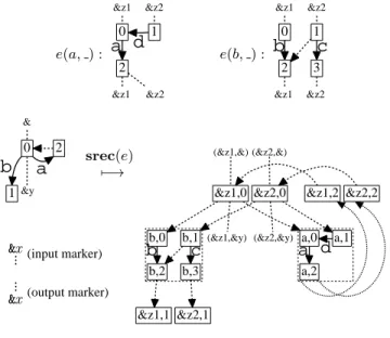
A picture of the bulk semantics for ordered graphs is given in Figure 7. As seen in the picture, with bulk semantics first we calculate the application of a given input functionf to a pair of each edge and its following subgraph of an input graph. Then we connect the results in keeping with the shape of the original graph, usingε-edges.
Recall the record notationG= (G.V, G.B, G.I), which is used in the following.
Definition 20 (Bulk Semantics of Structural Recursion). LetTbe
a monad onSet. For a functione:L×DBY →DBZZ, a structural recursion functionsrec(e):DBXY → DB
Z×X
Z×Y is defined as the
following.
ForG = (V, B, I) ∈ DBXY, srec(e)(G)
def
= (V′, B′, I′) ∈ DBZZ××XY where
•V′def= (Z×V) + (Σ(l,v′)∈L×Ve(l, G|v′).V)
(Here, an element (&z, v) in the left set Z×V—Z-copy of nodes of G—is a “hub” of the new graph, for this case we use the label Hub(&z, v) below. While, on the right of “+” and further in the case of(l, v′)of the direct sum “Σ”, a node
uine(l, G|v′).Vis “a piece of bulk”; eachl-labeled edge to
v′inGis replaced with this subgraphe(l, G|v′).V, which is
represented by a dotted box in Figure 7. For this case, we use the labelBulk(l,v′)(u). )
•B′: (Z×V) + (Σ(l,v′)e(l, G|v′).V)→
T(Lϵ×
(
(Z×V) + (Σ(l,v′)e(l, G|v′).V))+ (Z×Y)
)
Hub(&z, v) 7→T(g)(lift(λx.(&z, x))(B(v)))
e(a, ) :
0 1
2
a d
&z1 &z2
&z1 &z2
e(b, ) :
0 1
2
b
3
c
&z1 &z2
&z1 &z2
&x
... (input marker)
...
&x (output marker)
0 2
a
1
b
&
&y
srec(e)
7−→
(&z1,&)
&z1,0
b,0 (&z1,&y) a,0
(&z2,&)
&z2,0
b,1 (&z2,&y) a,1 &z1,2 &z2,2
b,2
b
b,3
c
&z1,1 &z2,1
a,2
a d
Figure 7. Bulk Semantics of Structural Recursion
g:Z×(Lϵ×V+Y)→
Lϵ×
(
(Z×V) + (Σ(l,v′)e(l, G|v′).V)
)
+ (Z×Y) (&z,Edge(l, v′)) 7→
(ifl=ε) Edge(ε,Hub(&z, v′))
(ifl̸=ε) Edge(ε,Bulk(l,v′)((e(l, G|v′).I)(&z))
)
(&z,Outm(&y)) 7→ Outm((&z,&y))
Bulk(l,v′)(u) 7→ T(h)((e(l, G|v′).B)(u))
h:Lϵ×(e(l, G|v′).V)+Z→
Lϵ×((Z×V) + (Σ(l,v′)e(l, G|v′).V))+ (Z×Y)
Edge(l′, u′) 7→ Edge(l′,Bulk(l,v′)(u′))
Outm(&z) 7→ Edge(ε,Hub(&z, v′))
• I′: Z×X → (Z×V) + (Σ
(l,v′)e(l, G|v′).V)
(&z,&x) 7→ Hub(&z, I(&x))
Next we see how structural recursion preserves finiteness of graphs.
Proposition 21. LetT be a finitary monad. Structural recursion
function maps finite graphs to finite graphs; more precisely, for
e:L×DBfY →DBfZZand a finiteT-graphG, the accessible part ofsrec(e)(G)is finite.
Proof. SinceTis finitary, for each elementv∈V, there is a finite subsetEv⊆ Lϵ×V such thatB(v)∈T(Ev+Y). Let
Edef= (∪v∈VEv)∩(L×V)⊆ L×V,
then sinceV is finite, so is E, and B is decomposed through
T(E+Y)⊆T(Lϵ×V+Y). Then the accessible part ofsrec(e)(G)
is included in the finite set
V′′def= (Z×V) + (Σ(l,v′)∈Ee(l, G|v′).V)⊆V′,
i.e.,I′(Z×X)⊆V′′andB′(V′′)⊆V′′.
Now recall the notion of bisimilarity for higher order functions. The following is stronger result than that proved in [Buneman et al. 2000] even whenT=Pfin, because here bisimulation genericity is

![Figure 10. Bulk Semantics of Structural Recursion: An Example of srec(rc, foldr(++, []))](https://thumb-ap.123doks.com/thumbv2/123deta/8631252.449565/16.918.115.841.113.510/figure-bulk-semantics-structural-recursion-example-srec-foldr.webp)